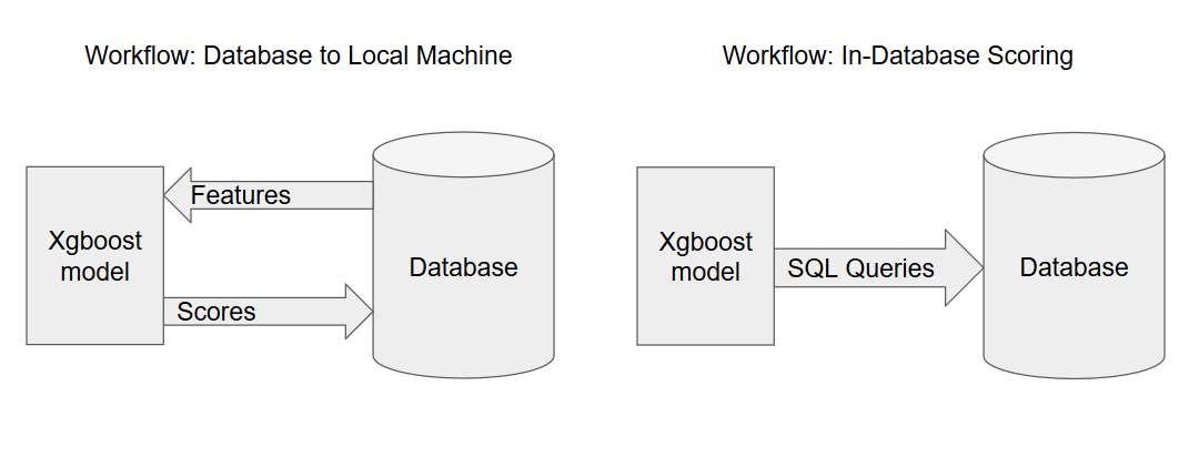
xgboost(docs) is a popular R package for classification and regression, and the model of choice in many winning Kaggle competitions. Moving xgboost into a large-scale production environment, however, can lead to challenges when attempting to calculate predictions (“scores”) for large datasets. We present a novel solution for calculating batch predictions without having to transfer features stored in a database to the machine where the model is located; instead we convert the model predictions into SQL commands and thereby transfer the scoring process to the database.
The enterprise problem arises when attempting to calculate probabilities for many thousands of subjects using many thousands of features located on a remote database. To run xgboost, the subject-features matrix must be loaded into memory, a cumbersome and expensive process.
Available solutions require using expensive high-memory machines or implementing external memory across distributed machines (expensive and in beta). Both solutions still require transferring all feature data from the database to the local machine(s), loading it into memory, calculating the probabilities for the subjects, and then transfering the probabilities back to the database for storage. In some of the author’s observed cases, 20-50 minutes for ~1MM subjects.

Local scoring vs. in-database scoring
A simple alternative is in-database scoring: we convert the xgboost model prediction process into a SQL query, and thereby accomplish the same task while leveraging a cloud database’s scalability to efficiently calculate the predictions.
To accomplish this, we’ll need to work through a few steps. First we’ll import the model as a list of nested tree structures that we can iterate through recursively. Then we’ll create a function that will recursively descend through a tree and translate it into a SQL CASE statement. We’ll then create a query that sums the CASE statements for all trees before logit-transforming it to calculate a probability.
First, let’s review how to convert the model object to a list of trees that we can work with:
library(xgboost)
library(jsonlite)
library(whisker)
# our model exists in the variable `xgb_model`:
# dump the list of trees as JSON and import it as `model_trees` using jsonlite
model_trees <- jsonlite::fromJSON(
  xgb.dump(xgb_model, with_stats = FALSE, dump_format='json'),
  simplifyDataFrame = FALSE)
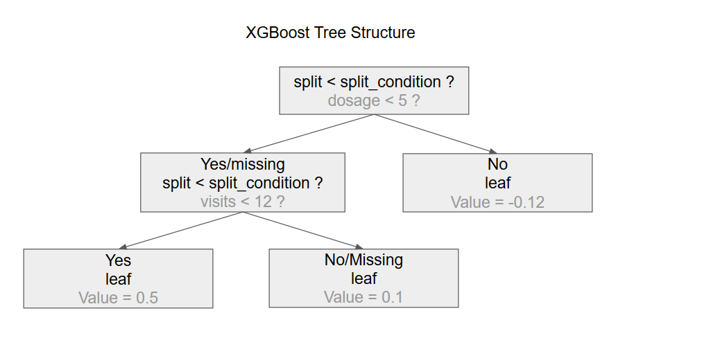
Now we need to translate each tree into a SQL CASE statement. Each tree represents a set of decisions based on a whether a variable (the ‘split’) is less than a threshold value (the ‘split_condition’). The result of the decision could be ‘yes’, ‘no’, or ‘missing’. In each case, the tree provides the ‘node_id’ of the next decision to evaluate. When we reach a leaf, no decision needs to be made and instead a value is returned. An example tree is shown below:

The structure of an xgboost tree
We’ll also need a dictionary that maps an integer to its associated feature name, since the trees themselves refer to 0-indexed integers instead of the feature names. We can accomplish that by creating the following list:
feature_dict <- as.list(xgb_model$feature_names)Using our feature_dict, we can recursively descend through the tree and translate each node into a CASE statement, producing a sequence of nested CASE statements. The following function does just that:
xgb_tree_sql <- function(tree, feature_dict, sig=5){
  # split variables must exist to generate subquery for tree children
  sv <- c("split", "split_condition", "yes", "no", "missing", "children")
  # we have a leaf, just return the leaf value
  if("leaf" %in% names(tree)){
    return(round(tree[['leaf']],sig))
  }
  else if(all(sv %in% names(tree))){
    tree$split_long <- feature_dict[[tree$split+1]] # +1 because xgboost is 0-indexed

    cs <- c(tree$yes, tree$no, tree$missing)
    cd <- data.frame(
      k = c(min(cs), max(cs)),
      v = c(1,2)
    )
    tree$missing_sql <- xgb_tree_sql(tree$children[[cd$v[cd$k==tree$missing]]], feature_dict)
    tree$yes_sql <- xgb_tree_sql(tree$children[[cd$v[cd$k==tree$yes]]], feature_dict)
    tree$no_sql <- xgb_tree_sql(tree$children[[cd$v[cd$k==tree$no]]], feature_dict)

    q <- "
      CASE
        WHEN {{{split_long}}} IS NULL THEN {{{missing_sql}}}
        WHEN {{{split_long}}} < {{{split_condition}}} THEN {{{yes_sql}}}
        ELSE {{{no_sql}}}
      END
    "
    return(whisker.render(q,tree))

  }

}
When we transform one tree into a sequence of nested case statements, we are producing a statement that yields that tree’s contribution to the total score. We now need to sum the output of each tree and then calculate the total probability prediction. In other words, we need to add up a list of nested CASE statements and then logit-transform the result.
Note that in the below we make use of the R ‘whisker’ package. This logic-less templating language is a great way to easily transform associative-arrays into SQL that contains easily identifiable labels as placeholderd. We find this more readable than sequences of ‘paste’ statements.
xgb_sql_score_query <- function(list_of_trees, features_table, feature_dict, key_field = "id"){

  # a swap list to render queries via whisker
  swap <- list(
    key_field = key_field,
    features_table = features_table
  )

  # score_queries contains the score query for each tree in the list_of_trees
  score_queries <- lapply(list_of_trees, function(tree){
    xgb_tree_sql(tree, feature_dict)
  })
  # the query clause to sum the scores from each tree
  swap$sum_of_scores <- paste(score_queries, collapse=' + ')

  # score query that logit-transforms the sum_of_scores
  q <- "
    SELECT
      {{{key_field}}},
      1/(1+exp(-1*( {{{sum_of_scores}}} ))) AS score
    FROM `{{{features_table}}}`
  "
  return(whisker.render(q,swap))
}
We are now ready to generate the score query from our model:
queries <- xgb_sql_score_query(
  model trees,
  'mydataset.my_feature_table',
  feature_dict
)
for(q in queries){
  # example: run the query with the R bigrquery package
  bq_project_query('my_project', q)
}
In summary, production models typically calculate predictions for all subjects on a daily, hourly, or even more frequent basis, however moving feature data between a database and a local “scoring” machine is expensive and slow. Transfering the scoring calculations to run within the database, as we’ve shown above, can significantly reduce both cost and run-time.
The astute reader may notice that, depending on the database, this will work for a limited number of trees. When that becomes a problem, it is possible to add another layer that stores the summed scores for batches of trees as views or tables and then aggregates their results. Beyond that, when queries with views become too long, it is possible to add an additional layer than aggregates batches of views into tables. These extensions are both left as an optional excercises for the reader.
Note: Since xgboost converts data internally to 32-bit, this procedure assumes that the data you are working with are stored as 32-bit floats. See https://github.com/dmlc/xgboost/issues/4097.