Understanding how Optimizely Controls Error in A/B Tests with R Part 1

Illustrating alpha and beta parameters

Let’s try to illustrate this through a simulation. We’ll simulate two sequences of conversions with conversion rates such that cr_b = (1+mde)*cr_a. We’ll then run a t-test comparing all of the available observations of the two groups each time we have a new pair of observations. If the p-value of the t-test is below 5%, we will reject the null-hypothesis that there is no difference between the distributions; hence, p.value < 0.05 implies there is a statistically significant difference between the conversion rates. Finally we’ll plot 1-p.value to represent “confidence” relative to where we are in the sequence. This essentially simulates what p-values we would calculate if we were to continually monitor conversions as subjects choose to convert or abandon. We add the 95% confidence line horizontally, as well as a vertical line at n_obs, the number of observations our power calculation says to use to conduct a t-test.

library(ggplot2)
set.seed(2)

# make our "true" effect larger than the mde
effect <- mde
cr_b <- (1+effect)*cr_a
observations <- 2*n_obs

# a sequence of {0,1} conversions
conversions_a <- rbinom(observations, 1, cr_a)
conversions_b <- rbinom(observations, 1, cr_b)

# Calculate p-values at each simultaneous observation of the a and b groups
tt <- sapply(10:observations, function(x){
  t.test(conversions_a[1:x],conversions_b[1:x])$p.value
})

tt <- data.frame(p.value = unlist(tt))

# for plots
conf_95 <- data.frame( x = c(-Inf, Inf), y = 0.95 )
obs_limit_line <- data.frame( x = n_obs, y = c(-Inf, Inf) )

# plot the evolution of p-value over time, if "peeking"
ggplot(tt, aes(x=seq_along(p.value), y=1-p.value)) + 
  geom_line() + 
  geom_line(aes(x, y, color="alpha=5%"), linetype=3, conf_95) + 
  geom_line(aes(x, y, color="end of test"), linetype=4, obs_limit_line) +
  xlab("Observation (day)") +
  scale_color_discrete(name = "Legend") +
  ylim(c(0,1))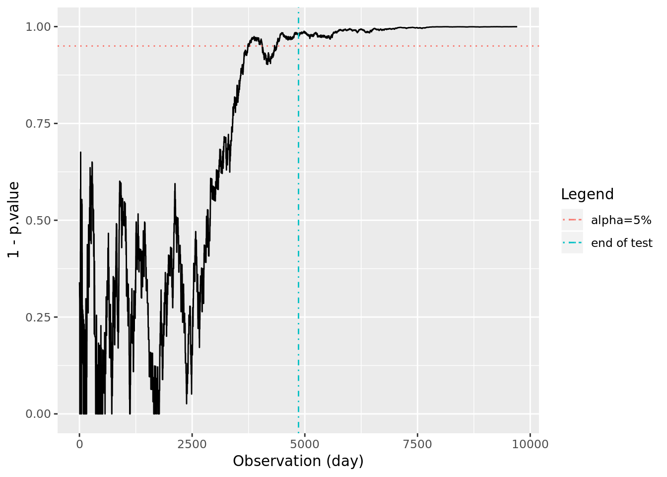

We observe that in the above example we would correctly have measured a difference in conversion rates for this particular simulation. However, we should expect that if we run this experiment 100 times, about 20 of those times will result in an incorrect negative prediction due to our false negative rate being 20% (power=80).

To test this, and many other concepts in this article, we are going to create a utility function that will run a simulation repeatedly:

#
# monte carlo runs n_simulations and calls the callback function each time with the ... optional args
#
monte_carlo <- function(n_simulations, callback, ...){
  simulations <- 1:n_simulations

  sapply(1:n_simulations, function(x){
    callback(...)
  })
}

Now, we’ll use the monte_carlo utility function to run 1000 experiments, measuring whether the p.value is less than alpha after n_obs observations. If it is, we reject the null hypothesis. We expect about 800 rejections and about 200 non-rejections, since 200/1000 would represent our expected 20% false negative rate.

reject_at_i <- function(observations, i){
  conversions_a <- rbinom(observations, 1, cr_a)
  conversions_b <- rbinom(observations, 1, cr_b)
  ( t.test(conversions_a[1:i],
           conversions_b[1:i])$p.value ) < alpha
}

# run the sim
rejected.H0 <- monte_carlo(1000, 
                           callback=reject_at_i,
                           observations=n_obs,
                           i=n_obs
                           )

# output the rejection table
table(rejected.H0)

## rejected.H0
## FALSE  TRUE 
##   190   810

We will use the same functions to test the false positive rate. In this case, we want to set the two conversion rates to the same value, cr_a and confirm that out of 1000 experiments, about 50 show up as having rejected the null hypothesis (and predict a difference in the conversion rates).

reject_at_i <- function(observations, i){
  conversions_a <- rbinom(observations, 1, cr_a)
  conversions_b <- rbinom(observations, 1, cr_a) # this is now the same conversion rate
  ( t.test(conversions_a[1:i],
           conversions_b[1:i])$p.value ) < alpha
}

# run the sim
rejected.H0 <- monte_carlo(1000, 
                           callback=reject_at_i,
                           observations=n_obs,
                           i=n_obs
                           )

# output the rejection table
table(rejected.H0)

## rejected.H0
## FALSE  TRUE 
##   962    38

Indeed, the results are as expected. We have shown that if we measure the results of our experiment when our power calculation tells us to, we can expect the false positive and false negative rates to reflect the values we have set in alpha and power.

Peeking

What happens if we don’t do a power calculation and instead monitor the conversions as they come in? This is what optimizely calls “peeking”. In other words, to run a test correctly you should only observe the results at one moment: when the power calculation has told you the test is complete. If you look at any moment prior to this, you are peeking at the results.

Peeking is widespread when it comes to analyzing experiments. In fact, some popular testing services peek continuously and automatically notify as soon as a p-value is below alpha. What you may notice, however, is that p-values can fluctuate around alpha multiple times before “choosing” a side. Continuously monitoring p-values will inflate false positive rates, up to 30%, Optimizely claims. Let’s see what effect continuous peeking has on our false positive rates:

peeking_method <- function (observations, by=1){
  # create the conversions
  conversions_a <- rbinom(observations, 1, cr_a)
  conversions_b <- rbinom(observations, 1, cr_a)  # no effect

  reject <- FALSE;

  # for each simulation, calculate the running conversion rates and days to complete.
  # Break the first time we have run more than the required days to complete
  for (i in seq(from=by,to=observations,by=by)) {
    tryCatch(
      {
        reject <- ( t.test(conversions_a[1:i],conversions_b[1:i])$p.value ) < alpha
        if(reject){
          break;
        }
      }, error=function(e){
        print(e)
      }
    )
  }
  
  reject

}
# run the sim
rejected.H0 <- monte_carlo(1000,
                           callback=peeking_method,
                           observations=n_obs,
                           by=100
                           )


# output the rejection table
table(rejected.H0)

## rejected.H0
## FALSE  TRUE 
##   653   347

Indeed, even peeking every 100 sets of observations leads to an inflated false positive rate of about 30%! Peeking at test results to make decisions, and especially automating peeking to make decisions, is a big no-no.

In a subsequent article, we’ll explore what optimizely proposes to resolve the peeking issue.